Blog Research
Language Model Fingerprinting Requires Rethinking Watermark Teachers
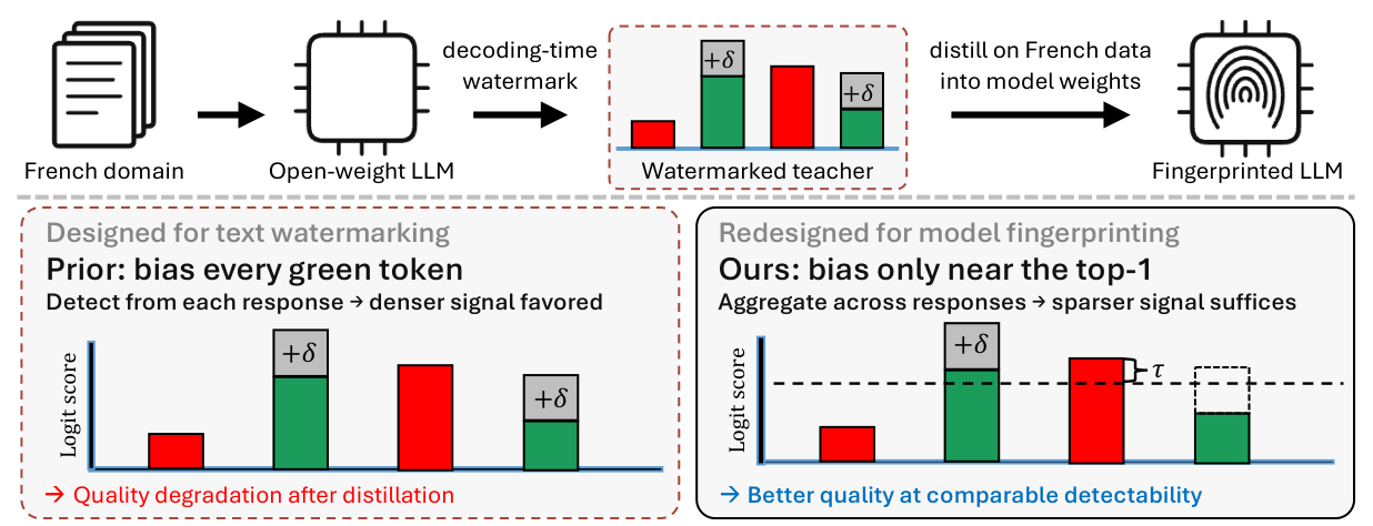
We rethink whether text watermarks are suitable distillation teachers for model fingerprinting. Aggregation across responses permits sparser signals; near-tie restriction places the bias on plausible tokens, improving generation quality at comparable detectability.
1POSTECH2University of Washington
Contents
Model fingerprinting for open-weight LLMs
As more capable LLMs are released with open weights, they can be deployed behind black-box APIs without honoring their licenses, raising concerns about model ownership and unauthorized use. A healthy open-weight ecosystem therefore needs reliable ownership verification that works from API responses alone. Black-box fingerprinting serves this purpose: it embeds a recognizable signal in the model before release so the owner can later test for it.
We focus on watermark-based fingerprinting (Gloaguen et al., 2026), which encodes the signal as a statistical pattern in responses from a secret fingerprint domain, such as French. Compared with backdoor fingerprints based on secret fixed trigger–response pairs, it produces more natural-looking outputs and better withstands deployment transformations, e.g., pruning, quantization, and fine-tuning.
How watermark-based fingerprinting works
Watermark-based fingerprinting builds on KGW, a widely used LLM watermarking scheme. Using a secret key and the previous h tokens, KGW pseudorandomly splits the vocabulary into green and red lists. It adds δ to green-token logits, making these tokens more likely to appear.
For a response \(x\) with \(L\) tokens, the detector compares the observed green count \(N_G(x)\) with the null expectation \(\gamma L\), where \(\gamma\) is the green-list fraction:
\[z(x) = \frac{N_G(x) - \gamma L}{\sqrt{\gamma(1-\gamma)L}}.\]A one-sided test declares the text watermarked when \(z(x) > \rho\).
For open-weight models, the owner cannot enforce this decoding rule after release. Fingerprinting therefore distills the KGW-biased teacher’s distribution into the model’s weights using data from a secret semantic domain (e.g., French), enabling the signal under ordinary decoding.
To verify model ownership, the owner queries a suspect model with prompts from this domain and aggregates its responses. The same test is applied after deduplicating context–token pairs, with green-list membership checked in each token’s original context.
Detection threshold and deployment changes
Our experiments use h = 1 and γ = 0.25. The detection threshold ρ = 4 corresponds to a nominal one-sided false-positive rate of approximately 3 × 10⁻⁵. We also test changes to sampling, system prompts, and model weights (quantization, pruning, and fine-tuning). The worst-case z-score is the lowest mean score across these transformations, with each mean computed over five seeds.
Prior evaluation understates the quality cost
Legitimate users also rely on the model within its fingerprint domain, so fingerprinting should preserve generation quality there. The prior evaluation reports accuracy on the French Benchmark and a metric labeled “PPL” that is actually mean token entropy. These metrics understate the degradation we observe in open-ended generation.
We reproduce the Llama-3.1-8B-Instruct setting (KGW, δ = 4) on 500 WritingPrompts prompts translated into French. Qwen-2.5-32B measures perplexity as an external reference model, and GPT-5 scores grammar, fluency, and coherence on a 1–10 scale. Figure 3 reports absolute perplexity; subsequent results use the ratio to the base model’s perplexity.
Prior utility evaluation
Our evaluation: open-ended generation · 500 French stories
Llama-3.1-8B-Instruct · KGW, δ = 4 · Each panel uses its own scale.
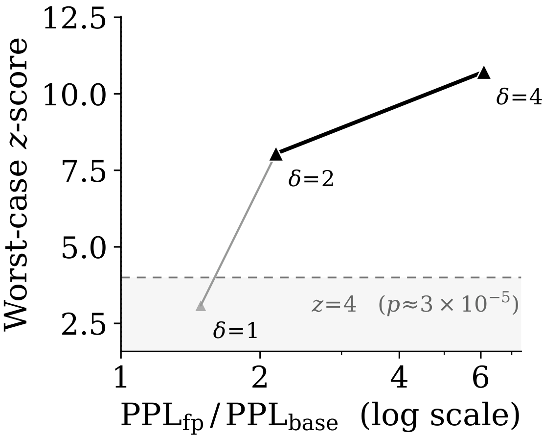
Reducing the bias improves quality at the expense of detectability. On Llama-3.1-8B, δ = 2 still yields a PPL ratio of 2.16, while δ = 1 falls below the worst-case detection threshold. Lowering δ alone does not recover near-base quality with reliable detection in this sweep.
Rethinking watermark teachers
Prior work uses a decoding-time text watermark as the distillation teacher.
Aggregation reduces the signal needed per response
Text watermarks are typically designed to remain detectable from an individual output, even when it is short or has been modified. In contrast, model fingerprinting allows aggregating evidence across responses, so each response can carry a weaker signal.
Where should the sparse signal be placed?
We favor green tokens that the base model already considers plausible. We analyze this choice through token surprisal: less probable tokens have higher surprisal.
To separate placement from teacher strength, we fix the base distribution and bias δ and compare green subsets with equal base probability mass. The resulting teachers have identical green-token probability and KL divergence from the base model. Yet the subset with lower average surprisal produces a smaller shift in expected base-model surprisal (Proposition 5.1).
Proposition 5.1: conditions and equations
At decoding step \(t\), let \(Q_t\) be the base distribution and \(G_t\) the green list. For a subset \(S \subseteq G_t\), \(\widetilde Q_t^S\) denotes the teacher obtained by adding bias \(\delta\) to the logits of tokens in \(S\).
The base-model surprisal of a token and the probability-weighted average within \(S\) are
\[\begin{aligned} r_t(v) &= -\log Q_t(v), \\ \bar r_t(S) &= \mathbb{E}_{v\sim Q_t(\cdot\mid S)}[r_t(v)]. \end{aligned}\]The teacher’s surprisal shift is the change in expected base-model surprisal:
\[\begin{aligned} \Delta_t^{\mathrm{surp}}(\widetilde Q_t^S; Q_t) &= \mathbb{E}_{v\sim\widetilde Q_t^S}[r_t(v)] \\ &\quad - \mathbb{E}_{v\sim Q_t}[r_t(v)]. \end{aligned}\]Proposition 5.1. Suppose \(S_1,S_2\subseteq G_t\) satisfy \(Q_t(S_1)=Q_t(S_2)>0\) and receive the same bias \(\delta>0\). Their teachers have identical green-token probability and KL divergence:
\[\begin{aligned} \widetilde Q_t^{S_1}(G_t) &= \widetilde Q_t^{S_2}(G_t), \\ \mathrm{KL}(\widetilde Q_t^{S_1}\Vert Q_t) &= \mathrm{KL}(\widetilde Q_t^{S_2}\Vert Q_t). \end{aligned}\]Their surprisal shifts, however, are ordered by the subsets’ average surprisal:
\[\begin{gathered} \Delta_t^{\mathrm{surp}}(\widetilde Q_t^{S_1}; Q_t) \le \Delta_t^{\mathrm{surp}}(\widetilde Q_t^{S_2}; Q_t) \\ \Longleftrightarrow\quad \bar r_t(S_1)\le\bar r_t(S_2). \end{gathered}\]Thus, at matched strength, biasing the subset with lower average surprisal produces a smaller surprisal shift.
This motivates near-tie restriction: biasing only green tokens close to the base model’s top prediction.
Near-tie restriction
We measure closeness to the top prediction by the logit gap, which is also the difference in surprisal.
Let \(\ell_t\) be the base model’s logits and \(v_t^\star\) its top-1 token. Because the softmax normalizer cancels, a token’s surprisal \(r_t(v) = -\log Q_t(v)\) under the base distribution \(Q_t\) exceeds that of the top-1 by exactly its logit gap:
\[r_t(v) - r_t(v_t^\star) = \ell_t(v_t^\star) - \ell_t(v).\]The teacher applies the bias only to green tokens whose gap is below τ:
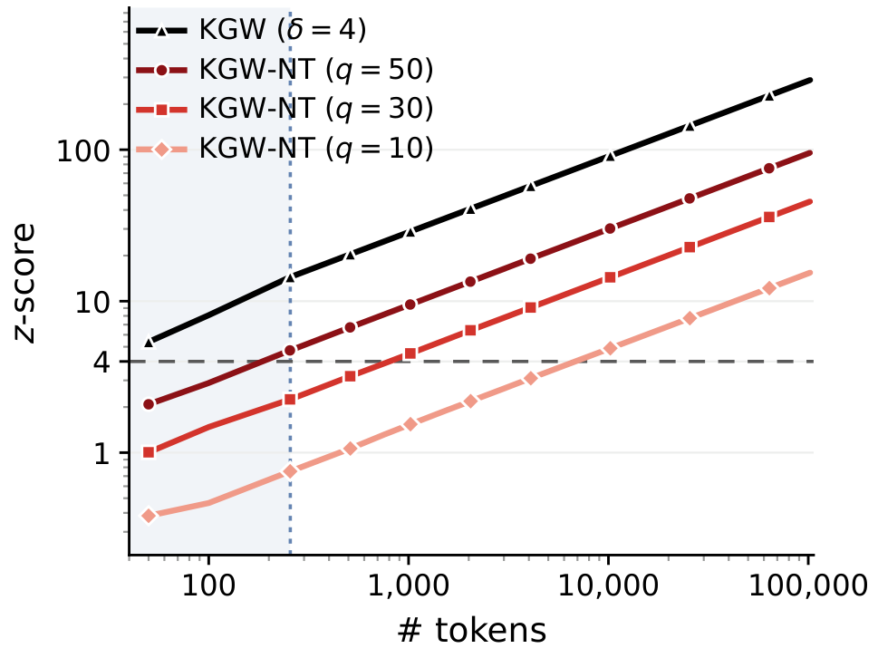
\[S_t^{\mathrm{NT}}(\tau) = \{v \in G_t : \ell_t(v_t^\star) - \ell_t(v) < \tau\}.\]Applying this restriction to KGW gives KGW-NT. We set τ to the q-th percentile of top-1–top-2 logit gaps on the fingerprint training data. Smaller q gives a sparser teacher, and τ → ∞ recovers KGW.
Which green tokens receive the bias?
“Le chat dort sur le ___” (The cat sleeps on the ___.)
Illustrative logits, not measured model outputs. The top-1 is canapé (sofa); fauteuil, lit, and tapis are plausible substitutes, and 4 of the 10 candidates are on the green list.
Near-tie biases 2 of 4 green tokens; δ = 4.0, τ = 1.2.
Teacher distribution statistics
Changing τ changes the biased mass as well as token selection. This demo illustrates the restriction; Table 2 in the paper tests placement at matched mass. These teacher statistics do not measure student quality.
After distillation, near-tie also yields lower PPL ratios than random green subsets matched in base probability at every position:
| Calibration percentile q | Random placement: PPL ratio ↓ | Near-tie: PPL ratio ↓ |
|---|---|---|
| 30 | 1.11 ± 0.04 | 1.02 |
| 50 | 1.25 ± 0.02 | 1.04 |
Llama-3.1-8B, δ = 4; three random placements per setting.
The detector selects positions using the base model. The owner re-scores each response using their own model, keeps positions whose top-1–top-2 gap is below τ, and computes the green-token z-score after deduplication. Selection does not use the secret key or green list, preserving the null green-token rate γ. We use the same detection threshold.
Tokens vs. positions in the detector
Teacher bias and detector selection are distinct: a green top-1 token receives the bias even when the runner-up lies outside τ, but the detector excludes such positions because selecting them by the top-1 token’s color would depend on the secret key. Position selection and the removal of repeated token pairs are both key-independent, which preserves the null rate; Appendix D of the paper analyzes the null variance and reports an empirical calibration check.
Results
- Models. Llama-3.2-3B, Qwen-2.5-3B, Llama-3.1-8B, Gemma-2-9B (instruct); the original French setup. Verification uses 1,000 French Alpaca queries with responses capped at 200 tokens.
- Baselines. KGW · SWEET (bias only at high-entropy positions) · MorphMark (adaptive bias strength) · KGW-TK (bias green tokens within the top-k; the rank-based control).
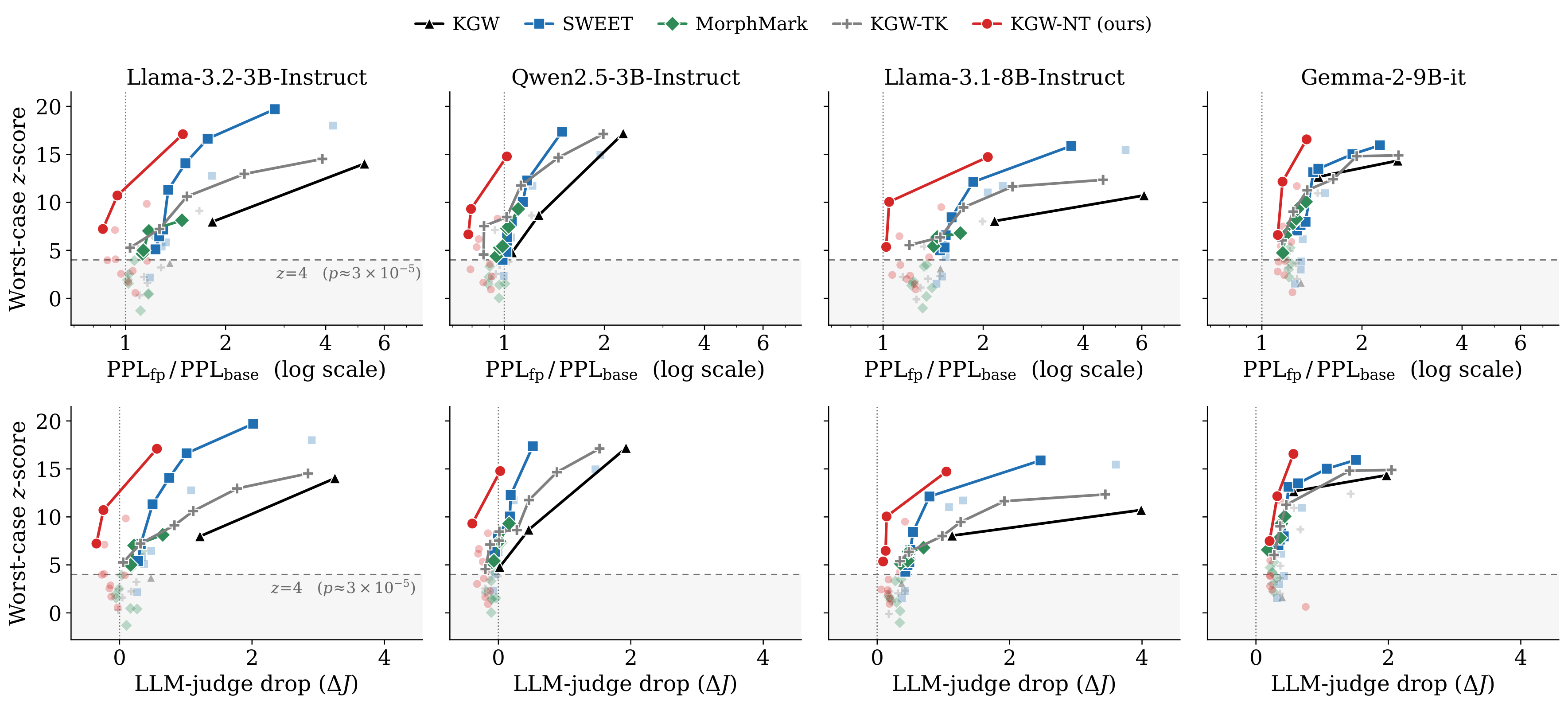
- Metrics. Quality: PPL ratio and LLM-judge drop on French WritingPrompts. Detectability: worst-case z-score over {sampling temperatures, system prompts, FP8/INT4 quantization, 50% pruning, French fine-tuning}, each averaged over five seeds.
Result 1: near-base quality at comparable detectability
| Teacher (Llama-3.1-8B) | PPL ratio ↓ | Judge score ↑ | Worst-case z-score ↑ |
|---|---|---|---|
| KGW, δ = 4 | 6.09 | 3.52 | 10.72 |
| KGW, δ = 2 | 2.16 | 6.40 | 8.05 |
| KGW-NT, q = 50, δ = 4 | 1.04 | 7.40 | 10.05 |
Tables 4–5 of the paper (base judge 7.51, KGW δ = 4 judge 3.52). Figure 3 uses Table 1 (base 7.76, KGW 3.73), which the paper reports separately.
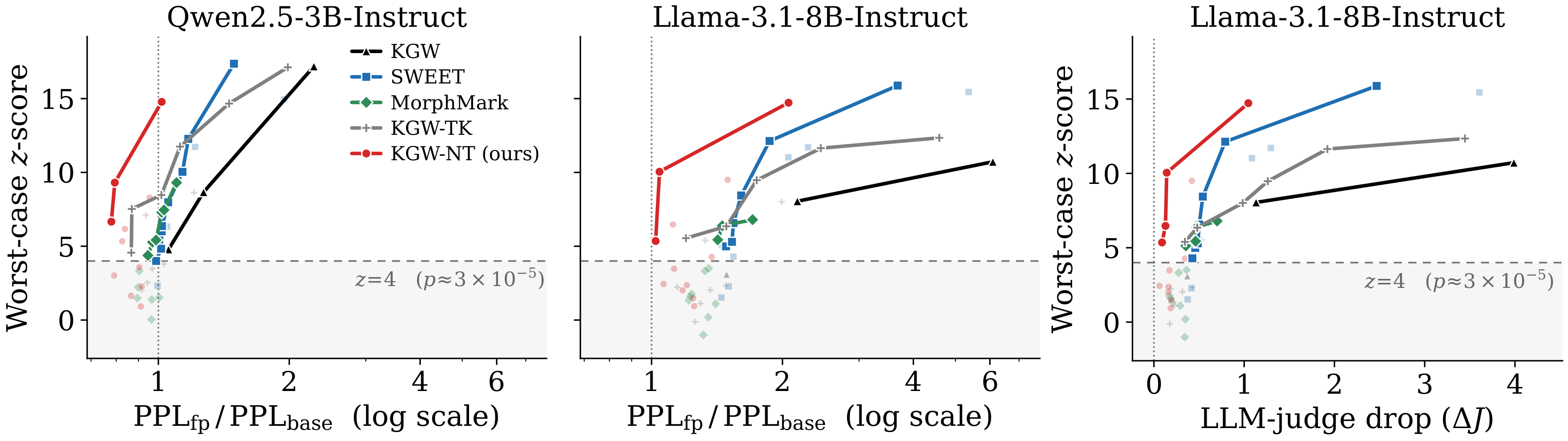
Across the frontier, KGW-NT reaches higher worst-case z-scores at the same PPL ratio and the same LLM-judge drop, or lower degradation at the same detectability. The gain over KGW-TK shows that sparsity alone is not the explanation: a top-k cutoff can still admit tokens with large logit gaps. On Llama-3.1-8B, KGW-TK and KGW-NT (q = 30, δ = 4) have similar output entropy (1.05 vs. 1.03) but PPL ratios of 1.20 vs. 1.02.
All four models and both quality metrics
Result 2: query-efficient detection at low distortion
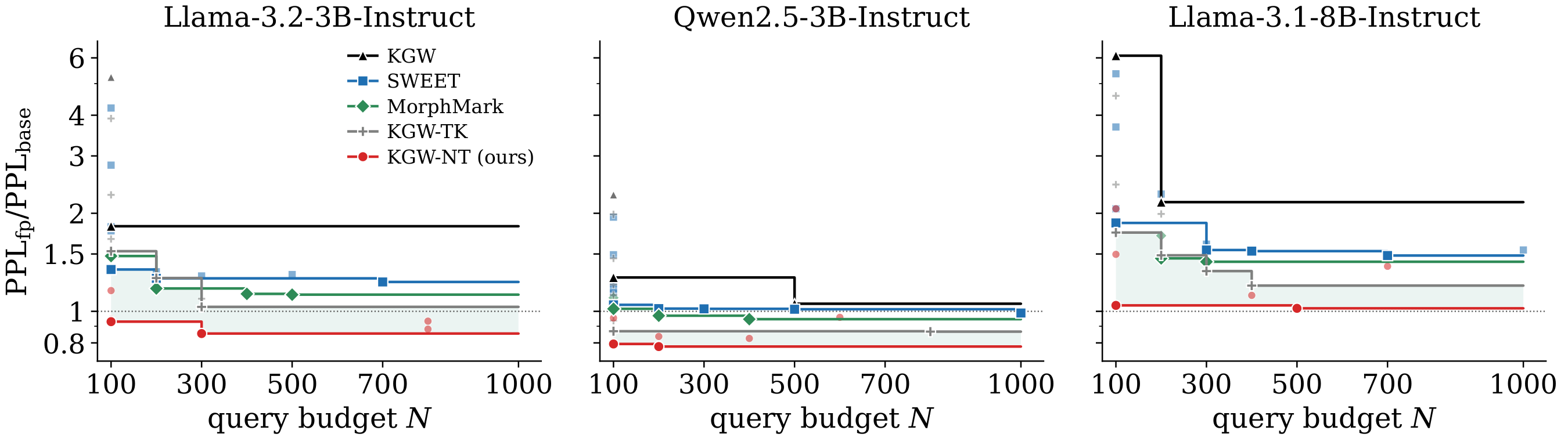
For each method and query budget N, we report the lowest PPL ratio among trained configurations whose worst-case z-score exceeds 4 within N queries. KGW-NT achieves the lowest PPL ratio at every evaluated budget. Larger budgets make sparser configurations detectable.
Result 3: near-tie combines with existing watermarking schemes
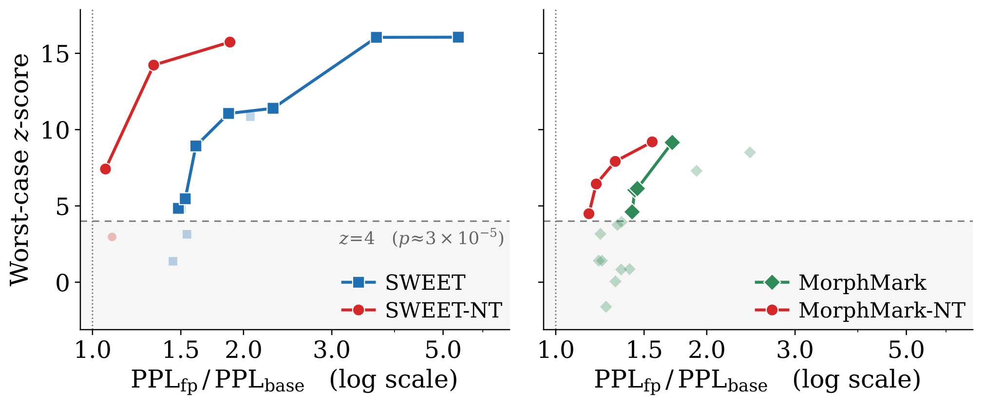
Near-tie restricts the tokens receiving the bias. It can therefore be combined with SWEET’s selection of generation positions or MorphMark’s adaptive bias strength. Both combinations improve the detection–quality frontier in our evaluation.
Conclusion
Prior utility evaluation understates what watermark-based fingerprinting costs in generation quality. Because verification aggregates evidence across queries, the watermark teacher need not be dense, and at matched strength the bias belongs on tokens the base model already finds plausible. Near-tie restriction applies this with a single logit-gap threshold. More broadly, watermark teachers for model fingerprinting should be designed for how fingerprints are verified, not inherited from text watermarking.
Citation
@article{hwang2026fingerprinting,
  title   = {Language Model Fingerprinting Requires Rethinking Watermark Teachers},
  author  = {Hwang, Jeongyeon and Nasery, Anshul and Oh, Sewoong and Ok, Jungseul},
  journal = {arXiv preprint arXiv:2610.04169},
  year    = {2026}
}